

When modeling a battery system, specifying a load profile is critical for accurately representing how the battery will operate in a real-world scenario. In the COMSOL Multiphysics® software and the Battery Design Module, several approaches are available to accommodate such profiles in your battery model. This blog post discusses these approaches and elaborates on their implementations. To demonstrate the use of these methods, we will review model examples from the Application Libraries in COMSOL Multiphysics®.
Introduction
You typically complete the construction of your battery model in the COMSOL® software by defining and prescribing the applied load, which may be based on the current, power, voltage, or a combination of these variables. Depending on the battery interface you use in your model, you can accomplish this by choosing the suitable boundary condition or operation mode and configuring the relevant value to match the operational requirements of the battery you aim to simulate.
For example, in the Lithium-Ion Battery, Battery with Binary Electrolyte, and Lead–Acid Battery interfaces, and for generic current distribution, you have a variety of options available for electrode conditions. Alternatively, in simplified battery interfaces like the Single Particle Battery and Lumped Battery interfaces, you can select an operation mode. At the pack level, in the Battery Pack interface, the load can be prescribed by setting the boundary conditions for the Current Conductor domains within a battery pack.
In COMSOL Multiphysics® and the Battery Design Module, several methods are available to capture and integrate the profile duration, variations, and cycle patterns into the expression you create and pass this information to the physics interface as the applied load. We will discuss these methods in the following sections.
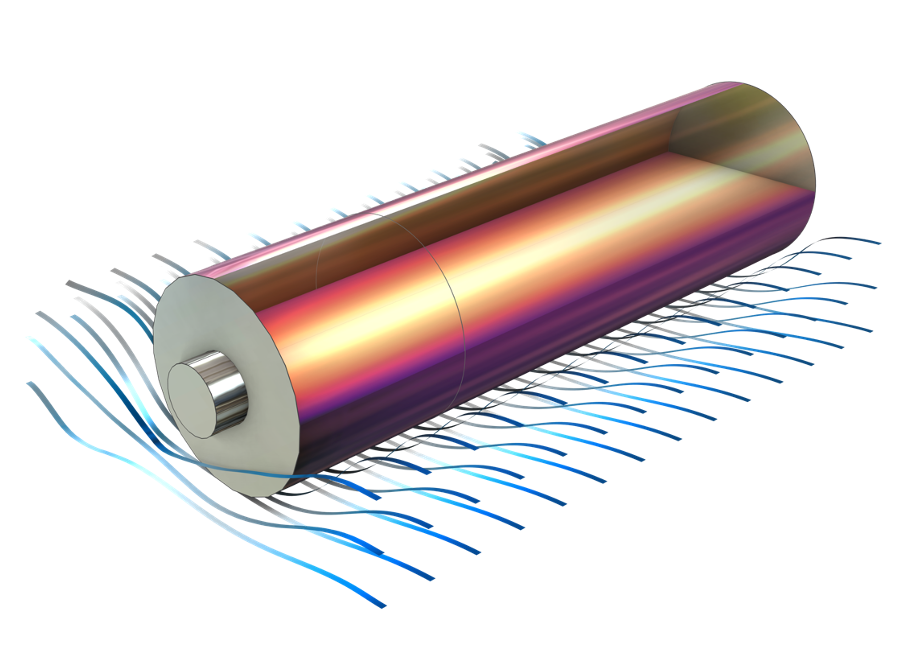
Temperature profile in an air-cooled cylindrical lithium-ion battery during a charge/discharge cycle.
Functions
Different functions within COMSOL Multiphysics® offer various choices for defining load profiles. By utilizing these functions, you can precisely capture the characteristics of the load profile, including patterns and variations over time. These functions can be incorporated into an expression representing the load, such as the applied current used in a battery model. For instance, in the 1D Isothermal Lithium-Ion Battery example model, the applied current that generates constant-current (CC) charge and discharge cycles, along with rest periods, is defined using a Piecewise function. This function is particularly useful for defining loads that change at known intervals.
Similarly, in the 1D Isothermal Zinc-Silver Oxide Battery example model, the Piecewise function is employed to define a discharge-current-density pulse profile. In the Thermal Modeling of a Cylindrical Lithium-Ion Battery in 2D and Thermal Modeling of a Cylindrical Lithium-Ion Battery in 3D example models, a square Waveform function is employed to establish an alternating charge–discharge current followed by a relaxation period. In the Soluble Lead–Acid Redox Flow Battery model, a load cycle consisting of charge, discharge, and rest phases is defined using three Rectangle functions. Depending on the inputs you have and your knowledge of the desired load cycle, you can use one or more of a function and/or combine multiple functions of different types to achieve the desired profile.
Abrupt changes or discontinuities in load profiles can lead to numerical instabilities. Therefore, it is crucial to enable smoothing in the function setting window when defining load profiles for various functions, to ensure convergence. The time-dependent solver is tasked with resolving the transition between load steps, as defined by the smoothing process.
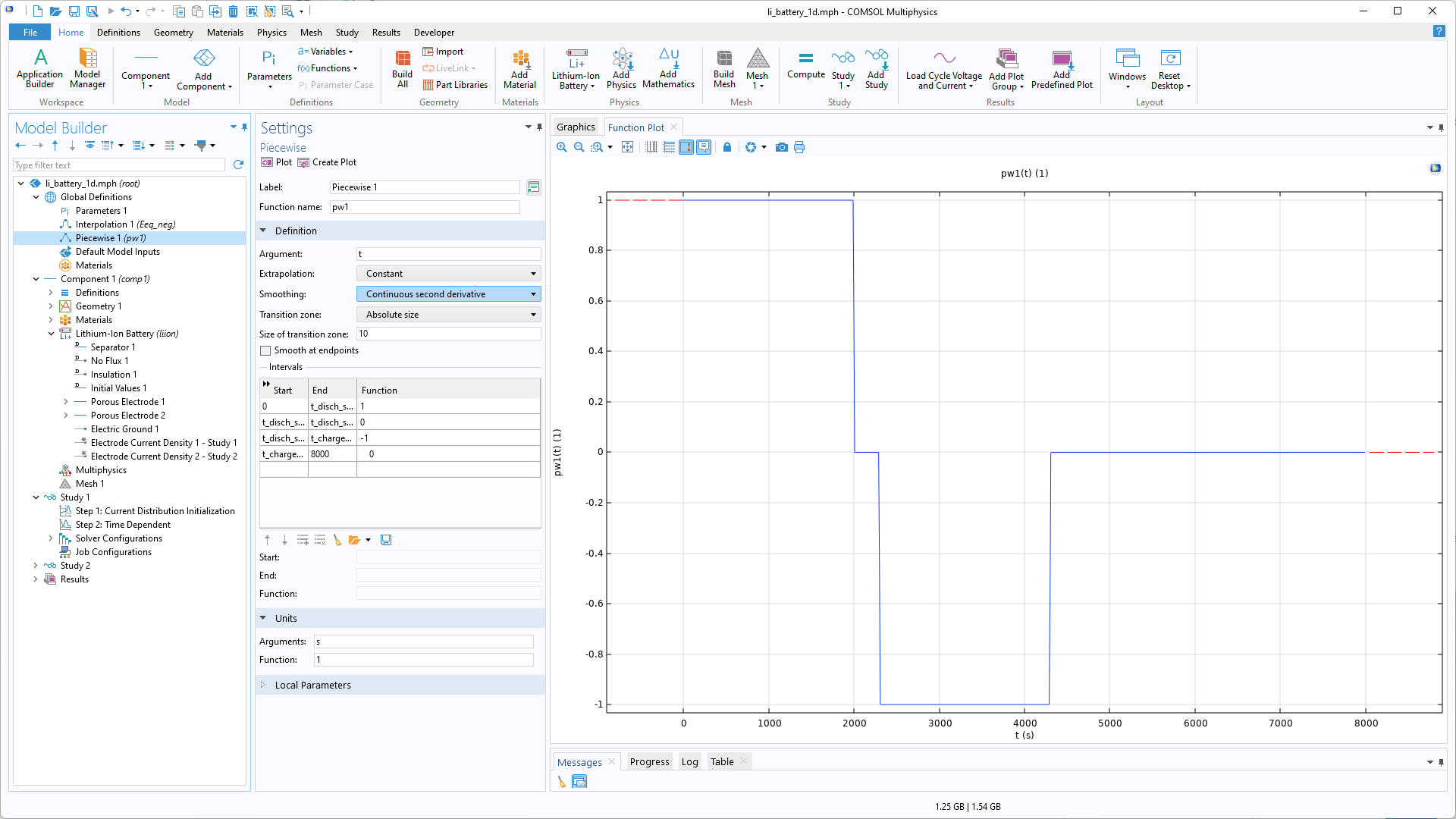
The Settings window for the Piecewise function, which defines a load profile, highlights the application of smoothing to improve the function’s numerical behavior.
Furthermore, if you have access to experimental load cycle measurements and want to incorporate the experimental load profile into your battery model, you can use an Interpolation function to import the data into COMSOL Multiphysics®. This capability is demonstrated in the Parameter Estimation of a Time-Dependent Lumped Battery Model example, where the experimental dynamic load data for a plug-in hybrid vehicle battery serves as the applied load to the Lumped Battery interface.
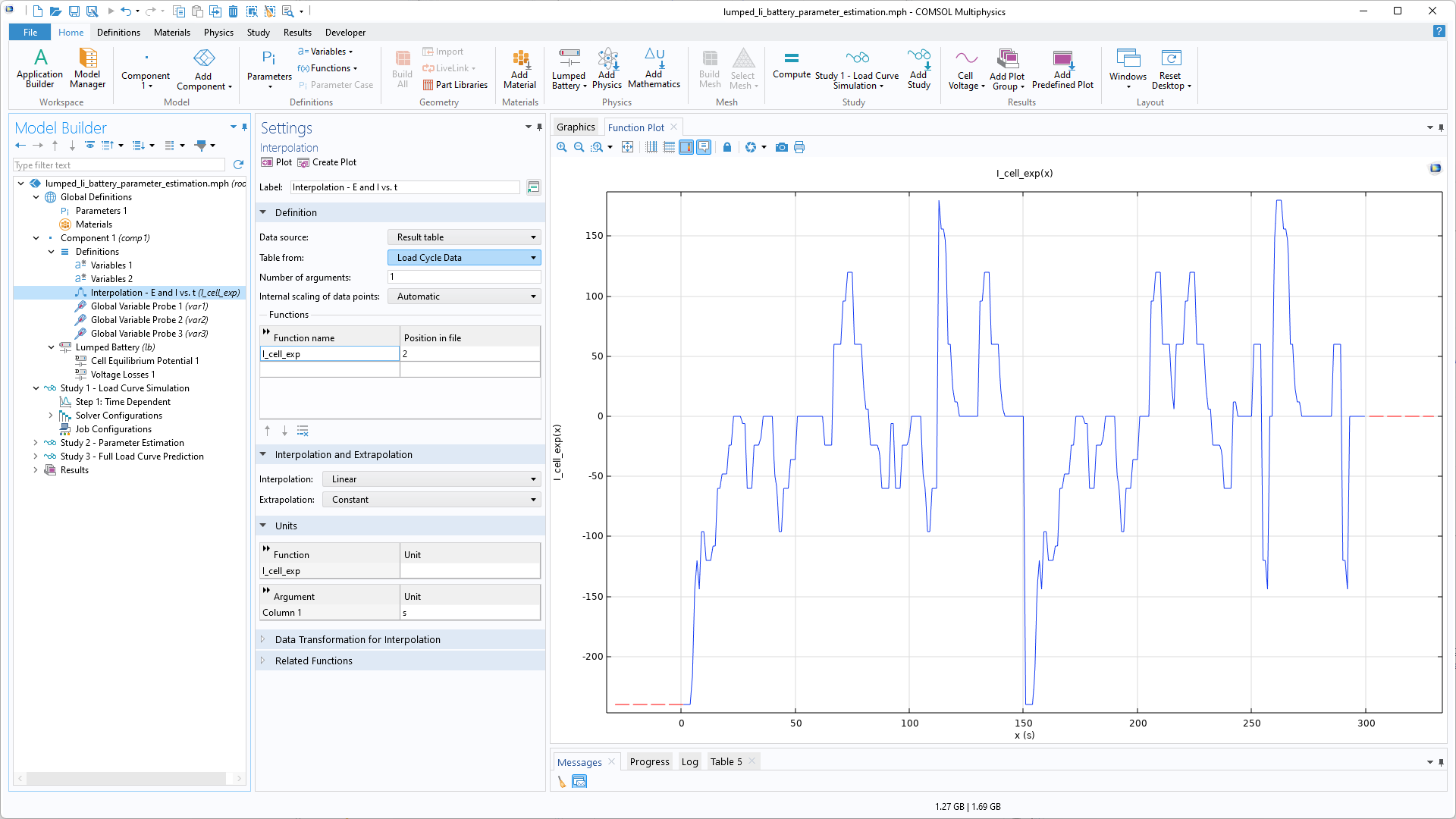
Experimental drive-cycle data is imported into COMSOL Multiphysics® through an Interpolation function to define the applied load.
Predefined Charge-Discharge Cycling Feature
If you intend to define a constant-current/constant-voltage (CCCV) cycling profile, you can use the predefined Charge-Discharge Cycling feature, which can be found in all battery and generic electrochemistry interfaces when using the Battery Design Module. This feature enables modeling of consecutive constant-current and voltage charge and discharge cycles, with the option to include rest between cycles. As shown in the screenshot below, the user can customize the order of the modes, assign a rest period time, and set the voltage and current thresholds for the constant-current and constant-voltage modes, respectively. This predefined set of profiles is repeated for as long as the simulation time allows.
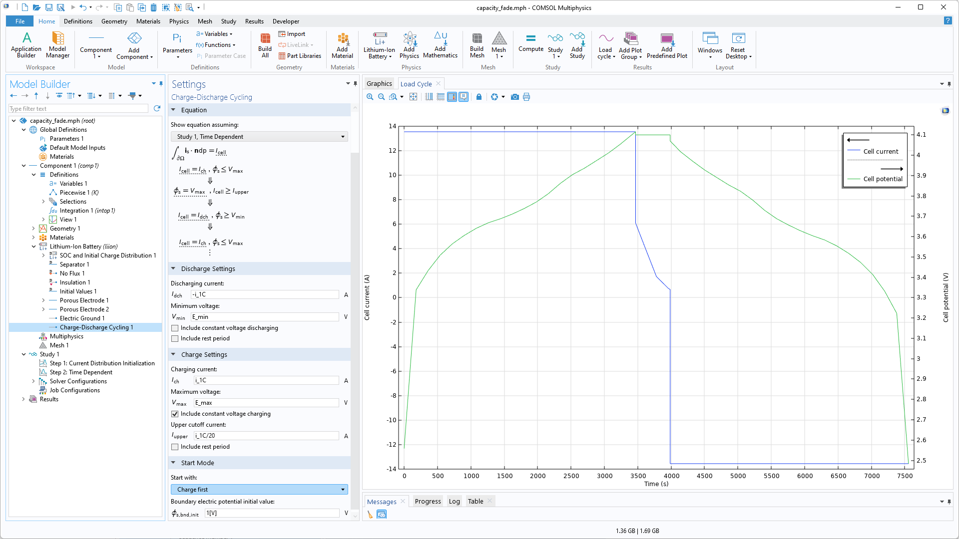
The Settings window for the Charge-Discharge Cycling node contains two separate sections for charge and discharge modes, allowing users to include or exclude steps in the profile and input the relevant values accordingly. Depending on the Start Mode setting, the node will begin the cycle with the Charge or Discharge mode.
The node also includes a cycle counter variable that can be accessed in the Results section or used to set a stop condition in the time-dependent solver. The Single Particle Model of a Lithium-Ion Battery and Capacity Fade of a Lithium-Ion Battery models use this feature to prescribe a CCCV profile.
The built-in node, Charge-Discharge Cycling, does come with certain limitations: It mainly relies on voltage and current thresholds to switch between modes, which may not fully align with your requirements. For more complex load cycles, you should consider configuring the cycling behavior using the Events interface.
Events Interface
It was mentioned earlier in the Functions section that applying smoothing while using different functions to define a load profile can enhance the solver’s numerical behavior during sudden load transitions. This enhancement is inherently integrated when defining a load profile using the Events interface, giving users confidence in the solver’s ability to maintain smooth numerical behavior. The Events interface enables battery modelers to create diverse loads with multiple steps and various criteria for mode switching. This is achieved by ensuring the load expression includes some switches defined via the Events interface, allowing the load expression to adopt different values, effectively reflecting the load profile pattern. The load expression is based on a number of discrete state variables that change value to define the desired load profile.
Before diving into how to use the Events interface to define your desired load profile, it’s essential to gain a better understanding of its key features. You can find the Events interface, under the Mathematics > ODE and DAE interfaces branch in COMSOL Multiphysics®. It primarily serves the purpose of creating solver events. These events can fall into two categories: explicit and implicit. Explicit events are predetermined to occur at specific times, such as the planned shutdown of the load at a designated moment. Implicit events come into play when certain conditions are met, like when the cell potential reaches a predefined cutoff threshold, necessitating a modification in applied current or placing the cell in a resting state. When an event occurs, the time-dependent solver halts, changes the values of one or several discrete state variables, and then restarts. It’s worth noting that the Charge-Discharge Cycling feature operates based on events, with implicit events already predefined “behind the scenes”.
To learn more about the Events interface and its practical implementation, you can explore the blog post Implementing a Thermostat with the Events Interface.
Now that we understand the workings of the Events interface, its key components, and how it enables users to modify their model based on specific conditions or at certain points, we can explore its use in defining load profiles. Different operational modes or steps in the load profile can be represented using a set of Discrete States. When these states receive different values, acting as a set of switches, they subsequently alter the definition of the load expression, as shown in the screenshot below. Deciding whether to use explicit or implicit events depends on the specifics of the load definition at hand. An explicit event can be employed if the timing of changes in variables that influence the profile pattern is known. In cases where the timing is unknown, the conditions and criteria signaling the onset of changes in these variables, such as specific thresholds for cell performance factors, can be detailed through a set of Indicator States. These Indicator States then establish state variables that the solver uses to trigger implicit events.
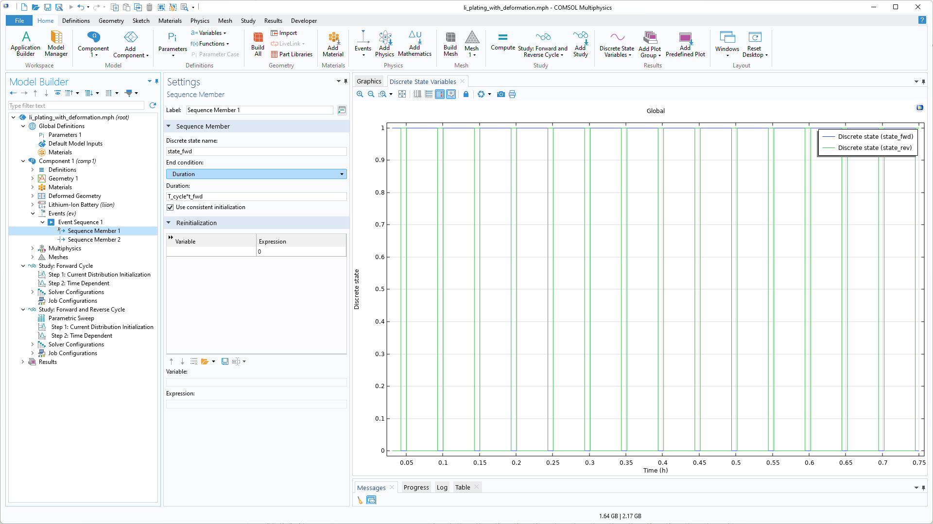
In the Lithium Plating with Deformation model, the Events interface is employed to create an Event Sequence that includes the duty cycles for forward and reverse currents.
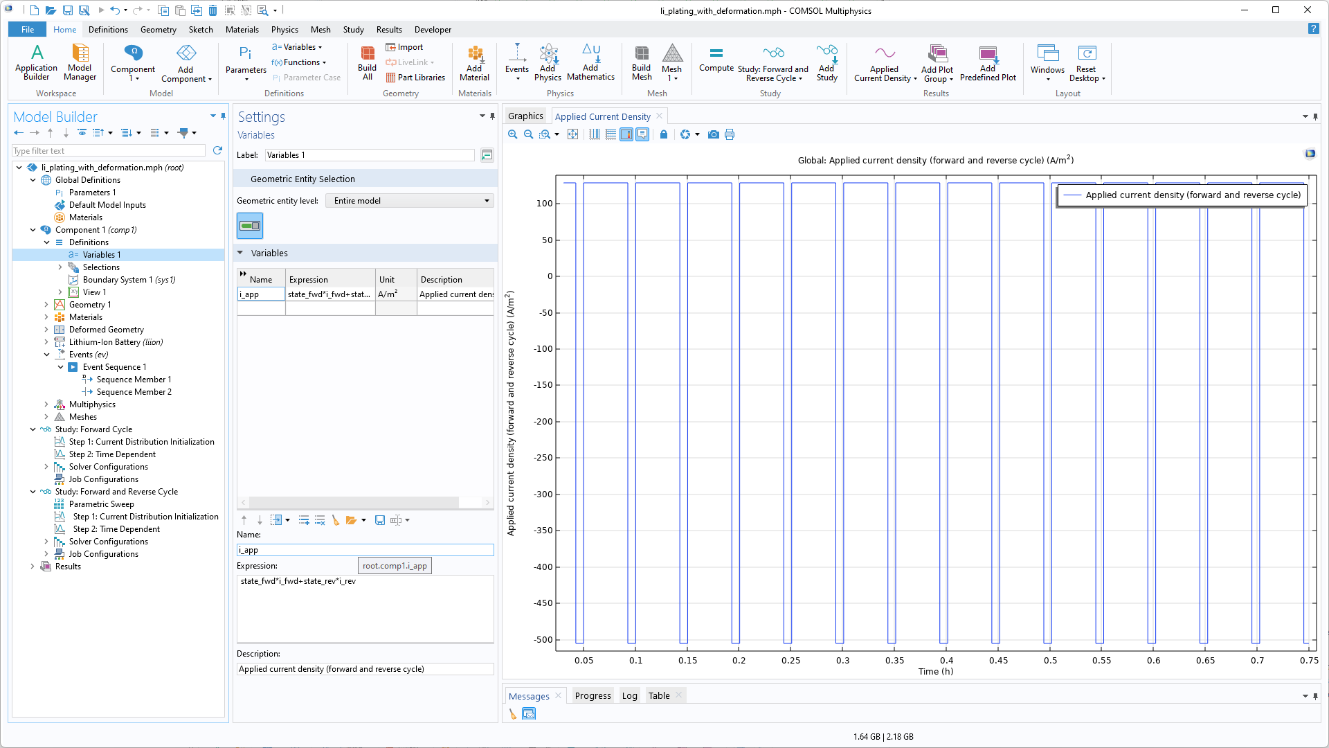
The applied electrode current density — defined as “i_app” in the Variables section and passed to the Electrode Current condition in the Lithium-Ion Battery interface — is computed by taking into account the forward and reverse states. This sequence is then looped, see the Settings window for the Event Sequence below.
Note that all Implicit Event and Explicit Event nodes are triggered at the specified time or when the condition is met. The order in which they are defined in the interface may not match the expected order of changes in the profile. However, another option, called Event Sequence, is available when right-clicking the Events interface, making it more straightforward to incorporate consecutive steps. By using an Event Sequence, you can specify a sequence of events that are activated in the order they are listed. Once an Event Sequence is added, you can include multiple sequence members, each operating based on conditional expressions or a specific duration. Furthermore, you can select the Loop check box in the Event Sequence setting window when using an Event Sequence. This allows events to be repeated as long as the simulation time permits, providing the flexibility to define repetitive cycles.
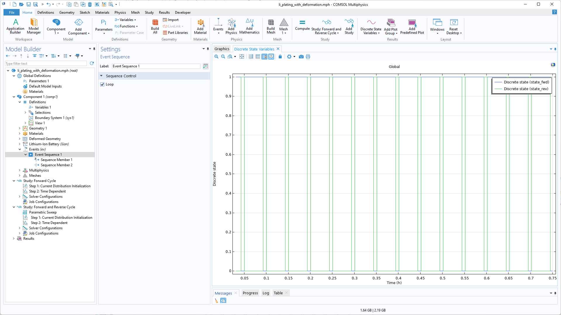
Choose the Loop check box if you want the event sequence to iterate repeatedly during the study, see the plot.
Implicit events can also terminate the simulation by setting up a Stop Condition for the solver at the point where the event occurs. This approach is often more precise than a stop condition defined through a Stop expression. As illustrated in the screenshot below, taken from the model Silicon-Graphite Blended Electrode with Thermodynamic Voltage Hysteresis, all implicit events defined in the model are automatically listed in the table, and simulation stops when any event marked as active is triggered.
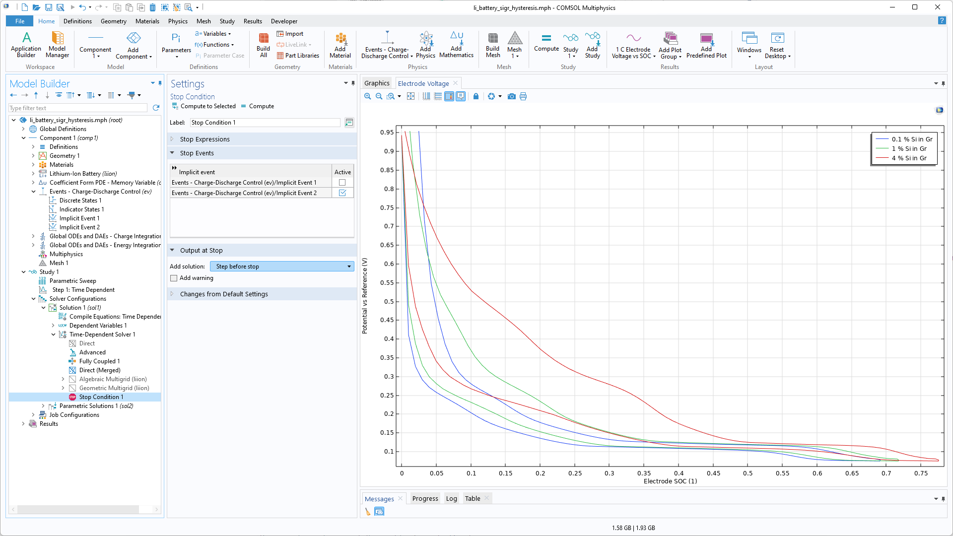
When the electrode potential exceeds the defined electrode potential corresponding to 0% electrode state of charge (SOC), Implicit Event 2 is triggered and signals the end of the simulation.
This approach is used in various battery models in COMSOL Multiphysics®, such as:
- Lithium Plating with Deformation
- Lithium Battery Designer
- Lithium-Ion Battery Internal Resistance
- Lithium-Ion Battery Rate Capability
- Battery Over-Discharge Protection Using Shunt Resistances
Concluding Remarks
In this blog post, we have explored various approaches users can employ to define a load cycle in COMSOL Multiphysics®. These methods are demonstrated in several model examples, which can serve as valuable resources for users to understand how they are applied within the context of battery simulations and gain insights into best practices and techniques for accurately representing load profiles in their simulation projects.


Comments (0)